This post is a compact English adaptation of two chapters from my bachelor's thesis. The original thesis text was written in German; this article translates and restructures the core ideas for blog format.

In short: Geometric Brownian Motion (GBM) is the baseline, and the Constant Elasticity of Variance (CEV) model is a useful extension when volatility should depend on the current price level.

Geometric Brownian Motion

Start directly from the stochastic differential equation

$$dS_t = \mu S_t\,dt + \sigma S_t\,dW_t.$$

Here, $\mu$ is drift, $\sigma$ is volatility, and $W_t$ is standard Brownian motion. Under this model, prices stay positive and $\log S_t$ is normally distributed.

In the thesis, GBM was also built from a discrete random-walk limit argument. That construction is still useful conceptually, but for practical calibration and simulation, the SDE form above is the working definition.

For rigorous background on Itô SDEs, existence, and stochastic integration, see ¹.

For daily observations $S_0,\dots,S_n$ with step size $\Delta t$, the log-returns

$$r_j = \log S_j - \log S_{j-1}$$

are approximately normal with

$$r_j \sim \mathcal N\!\left(\left(\mu-\tfrac12\sigma^2\right)\Delta t,\;\sigma^2\Delta t\right).$$

A practical estimator in R:

001log_returns <- diff(log(dax$Price))
002sigma <- sd(log_returns)
003mu <- mean(log_returns) + 0.5 * sigma^2

This gives immediate inputs for simulation, confidence intervals, and backtesting.

Brownian paths are almost surely not differentiable, so equations like

$$dS_t = a(S_t,t)\,dt + b(S_t,t)\,dW_t$$

must be read as integral equations,

$$S_t = S_0 + \int_0^t a(S_s,s)\,ds + \int_0^t b(S_s,s)\,dW_s.$$

This is the precise reason numerical schemes like Euler-Maruyama are used in implementations: they approximate these integrals on discrete time grids ^{1 2}.

Using the GBM closed form, a two-sided confidence interval for a horizon $T$ is

$$\left[S_0\exp\!\left((\mu-\tfrac12\sigma^2)T - z_{\alpha/2}\sigma\sqrt{T}\right), \;S_0\exp\!\left((\mu-\tfrac12\sigma^2)T + z_{\alpha/2}\sigma\sqrt{T}\right)\right].$$

R snippet:

001alpha <- 0.05
002T <- 252
003z <- qnorm(c(1 - alpha/2, alpha/2))
004ci <- S0 * exp((mu - 0.5 * sigma^2) * T + z * sigma * sqrt(T))

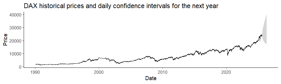
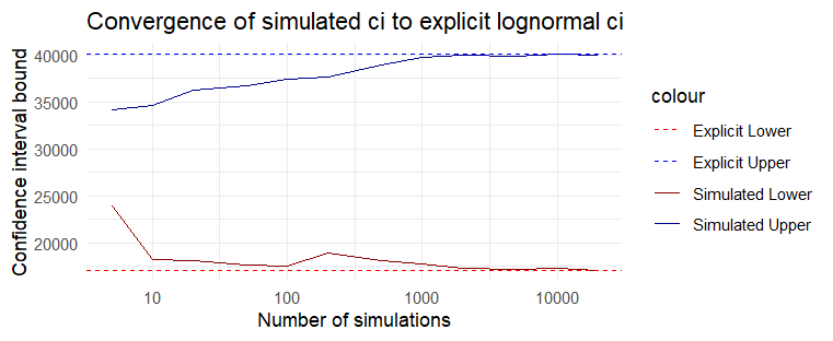
Monte Carlo approximates the same distribution numerically and is the bridge to models without closed forms ³.

001n <- 252
002paths <- 1000
003S0 <- tail(dax$Price, 1)
004
005simulations <- replicate(paths, {
006  W <- c(0, cumsum(rnorm(n, 0, 1)))
007  S0 * exp((mu - 0.5 * sigma^2) * c(0, 1:n) + sigma * W)
008})

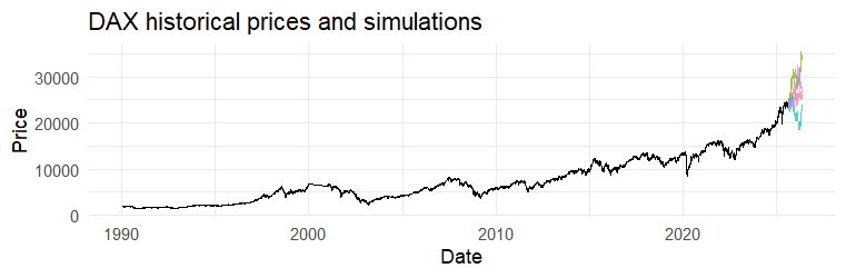
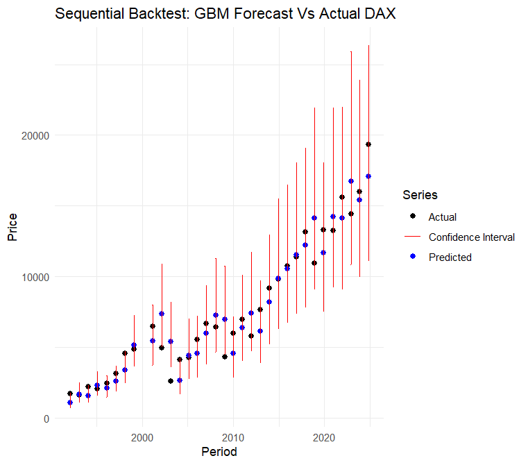
Backtesting answers a practical question: how often do realized values fall into model-based uncertainty bands?

In the thesis setup, calibration on one part of history and testing on a later part produced a coverage measure ("Überdeckungswahrscheinlichkeit" in the German text, translated as coverage probability).

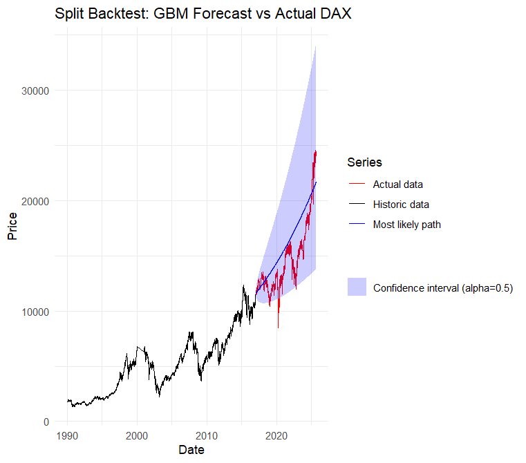
Sequential backtesting repeats this over rolling windows:

The confidence interval formula and Monte Carlo quantiles become closer as the number of simulated paths grows:

The CEV Model

This section corresponds to the second half of Chapter 7 of the thesis (translated from German).

CEV extends GBM by making diffusion state-dependent:

$$dS_t = \mu S_t\,dt + \sigma S_t^{\beta}\,dW_t.$$

Interpretation:

• $\beta = 1$: recovers GBM.
• $\beta < 1$: relatively higher volatility at lower prices.
• $\beta > 1$: volatility grows faster at higher prices.

So CEV can capture price-volatility coupling that GBM cannot.

For parameter estimation, a common route is Euler pseudo-likelihood (QMLE). With

$$\Delta S_i = S_{t_{i+1}} - S_{t_i},$$

the Euler step implies

$$\Delta S_i \mid S_{t_i} \approx \mathcal N\!\left(\mu S_{t_i}\Delta t,\;\sigma^2 S_{t_i}^{2\beta}\Delta t\right).$$

Hence the log-likelihood is approximated by

$$\ell(\mu,\sigma,\beta) = -\frac12\sum_{i=0}^{n-1} \left[ \log\!\left(2\pi\sigma^2 S_{t_i}^{2\beta}\Delta t\right) +\frac{(\Delta S_i-\mu S_{t_i}\Delta t)^2}{\sigma^2 S_{t_i}^{2\beta}\Delta t} \right].$$

Then maximize numerically under constraints like $\sigma>0$ and a bounded $\beta$ range.

This is the pseudo-maximum-likelihood route discussed in the thesis and in the SDE inference literature ².

Simulation (Euler-Maruyama):

001simulate_cev_paths <- function(S0, mu, sigma, beta, dt, nsteps, npaths) {
002  S <- matrix(NA, nrow = nsteps + 1, ncol = npaths)
003  S[1, ] <- S0
004
005  for (i in 1:nsteps) {
006    Z <- rnorm(npaths)
007    S[i + 1, ] <- S[i, ] + mu * S[i, ] * dt + sigma * (S[i, ]^beta) * sqrt(dt) * Z
008    S[i + 1, ][S[i + 1, ] <= 0] <- 1e-8
009  }
010
011  S
012}

Custom QMLE in R:

001estimate_cev <- function(S, dt = 1/252) {
002  S <- as.numeric(S)
003  dS <- diff(S)
004  S0 <- S[-length(S)]
005  eps <- 1e-12
006  S0[S0 <= 0] <- eps
007
008  init <- c(mu = 0.05, sigma = 0.2, beta = 1.0)
009
010  negloglik <- function(par) {
011    mu <- par[1]; sigma <- par[2]; beta <- par[3]
012    if (sigma <= 0 || beta <= 0 || beta >= 5) return(1e12)
013
014    denom <- (sigma^2) * (S0^(2 * beta)) * dt
015    denom[denom <= 0] <- eps
016
017    0.5 * sum(log(2 * pi * denom) + ((dS - mu * S0 * dt)^2) / denom)
018  }
019
020  res <- nloptr::nloptr(
021    x0 = init,
022    eval_f = negloglik,
023    lb = c(-Inf, 1e-8, 1e-6),
024    ub = c(Inf, Inf, 4.999),
025    opts = list(algorithm = "NLOPT_LN_SBPLX", xtol_rel = 1e-8, maxeval = 3000)
026  )
027
028  setNames(res$solution, c("mu", "sigma", "beta"))
029}

The optimizer setup above uses nloptr ⁴. A package-level alternative is Sim.DiffProc::fitsde ⁵. The custom estimator is competitive in comparison to the package.

A backtest for the CEV Model:

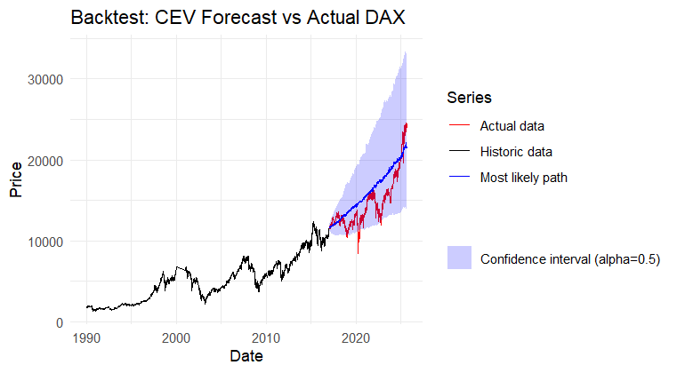
In this specific dataset, CEV can be close to GBM when $\beta$ is near $1$. In regimes where volatility strongly depends on level, CEV shows clearer gains.

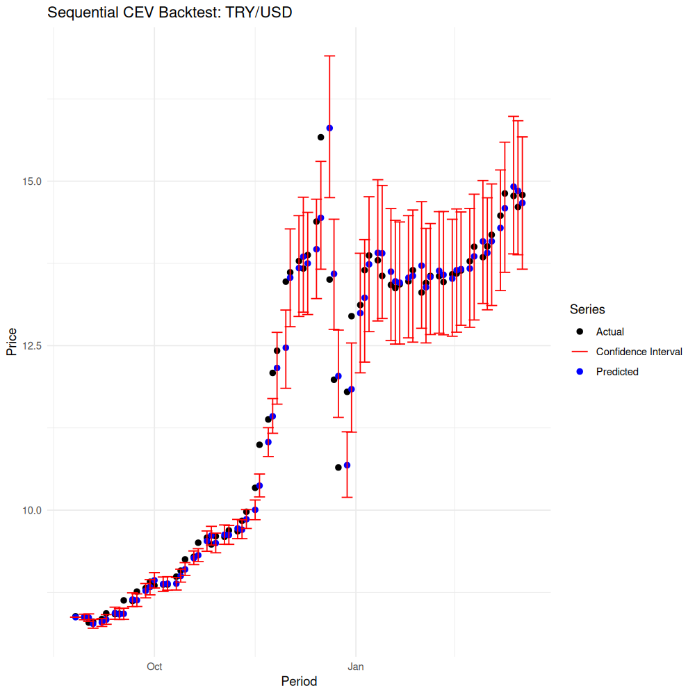
An example from the thesis is a stressed FX period:

Footnotes

1. Bernt Øksendal, Stochastic Differential Equations, Springer. Link ↩ ↩²

2. Stefano Iacus, Simulation and Inference for Stochastic Differential Equations. Link ↩ ↩²

3. Paul Glasserman, Monte Carlo Methods in Financial Engineering. Link ↩

4. nloptr package documentation. Link ↩

5. Sim.DiffProc package documentation. Link ↩